Simulation of Wave Functions in Quantum Mechanics

Simulation of Wave Functions in Quantum Mechanics#

(Cambridge Summer School’s Presentation)

written in jupyter notebook by Yiran Feng (Leon) 2025-08-02

1
Step = QMSim
2
Step.Gaussian = [-5, 0.5, 4]
3
Step.Potential = np.array([0] * 120 + [20] * 80)
4
%manim -qh Step

Introduction#

In chapter 2 and chapter 3, we’ve learnt about wave function in quantum mechanics and its characteristics, however, in a rather mathematical level, with equations and deductions. In this presentation, I’ll present you a python simulation of wave functions in different situations, giving you a intuitive way of understanding quantum mechanics.

For simplicity, all constants are set to one in this simulation, including mass, planck’s constant, etc.

1
# Libraries
2
import numpy as np
3
import scipy as sp
4
from matplotlib import pyplot as plt
5
from manim import *
6
from IPython.display import HTML
7
from copy import deepcopy as dc
8
from random import random
9
import tqdm
10

11
# Variables & Constants
12
inf = 100
13
x = np.linspace(-10, 10, 200)
14
y = np.linspace(-10, 10, 200)
15
X, Y = np.meshgrid(x, y)
16

17
# Useful functions
18
def find_nearest(array, value):
19
        array = np.asarray(array)
20
        idx = (np.abs(array - value)).argmin()
21
        return idx
22

23
def find_nearest_val(array, value):
24
        array = np.asarray(array)
25
        idx = (np.abs(array - value)).argmin()
26
        return array[idx]

Simulation on 1D#

Basically, the simulation consists of two parts: Initialization and Evolution.

Initialization#

The state of the system can be initialized with two functions: the initial state of the wave function and the potential function.

By considering different initial states of the wave function, we can change the position, the spread, and the momentum of the particle.

By changing the potential function, we can simulate different situations, for example, harmonic oscillator and quantum channel.

Look into the code. The class Simulation1D takes in two variables. phi_0 means the initial state of the wave function, and v defines the potential. The wave function is automatically normalised by the function _normalise, which is called inside the initialization, and probability ( which is basically $|\phi(x)|^2$ ) gives us the probability, of course.

1
class Simulation1D():
2
    def __init__(self, phi_0, v):
3
        self.phi = dc(phi_0); self.v = dc(v)
4
        self.dx = x[1] - x[0]; self.len = len(phi_0)
5
        self._normalise(); self._hamiltonian()
6
        self.prob = []; self.prob_updated = False
7

8
    def _normalise(self):
9
        self.phi /= np.linalg.norm(self.phi)
10
        self.prob_updated = True
11
        self.prob = (self.phi * self.phi.conjugate()).real
12

13
    def probability(self, pos = None):
14
        if not self.prob_updated:
15
            self._normalise()
16
        if pos:
17
            return self.prob[find_nearest(x, pos)]
18
        else:
19
            return self.prob

Evolution#

From chapter 2 and chapter 3, we’ve learnt that when a system is free from interactions with measuring devices, the evolution of the wave function can be calculated by the Schrödinger equation (44) (Postulate 6)

i\hbar \frac{\partial ψ(x,t)}{\partial t} = \left [ -\frac{\hbar ^ 2}{2m} \frac{\partial^2}{\partial x^2} + V(x) \right ] ψ(x,t)

In our cases, the mass and $\hbar$ is set to 1. Introducing the hamiltonian operator $\hat H$ , the 1-dimensional time-dependent Schrödinger equation (TDSE) can be deduced

\frac{\partial}{\partial t} ψ(x, t) = -i\hat H ψ(x, t)

where

\hat H = -\frac{1}{2} \nabla ^2 + V(x)

In this equation, the discrete Laplace operator can be given as convolution with the finite-difference kernel, $[1, -2, 1]$ , results in a symmetric Tridiagonal Toeplitz matrix with the finite-difference coefficients along the diagonals. Combining this matrix with the potential $V=[V_0, V_1, ..., V_N]$ , a full Hamiltonian operator in matrix form can be obtained

\hat H = -\frac{1}{2\Delta x^2} \begin{bmatrix} -2 & 1 & \quad & \quad & \quad \\ 1 & -2 & 1 & \quad & \quad \\ \quad & \quad & \ddots & \quad & \quad \\ \quad & \quad & 1 & -2 & 1 \\ \quad & \quad & \quad & 1 & -2 \\ \end{bmatrix} + \begin{bmatrix} V_0 & \quad & \quad & \quad & \quad \\ \quad & V_1 & \quad & \quad & \quad \\ \quad & \quad & \ddots & \quad & \quad \\ \quad & \quad & \quad & V_{N-1} & \quad \\ \quad & \quad & \quad & \quad & V_N \\ \end{bmatrix}

1
def _hamiltonian(self):
2
    """Returns Hamiltonian using finite differences."""
3
    L = [[0 for j in range(self.len)] for i in range(self.len)]
4
    for i in range(self.len):
5
        for j in range(self.len):
6
            if i == j:
7
                L[i][j] = -2
8
            if abs(i-j) == 1:
9
                L[i][j] = 1
10

11
    # Somehow it doesn't work...
12
    # L = sp.sparse.diags([1, -2, 1], offsets=[-1, 0, 1], shape=(self.len, self.len))
13

14
    L = np.array(L) / self.dx ** 2
15
    H = -L / 2 + sp.sparse.spdiags(self.v, 0, self.len, self.len)
16
    self.H = sp.sparse.csc_matrix(H)
17

18
Simulation1D._hamiltonian = _hamiltonian

If the Hamiltonian is independent of time, a time evolution operator(U) can be obtainted

ψ(t+\delta t) = Uψ(t)

where

U = e^{-i\hat H \delta t}

Multiplying the wave function with the operator $m$ times, we can advance the time steps to $t + m\delta t$

ψ(t+m\delta t) = U^mψ(t)

The code below calculates the time evolution operator based on the hamiltonian and dt, and applies the operator to the wave function, which is also normalized after the procedure.

1
def simulate(self, dt = 1e-3):
2
    """Generates wavefunction and time at the next time step."""
3
    U = sp.sparse.linalg.expm(-1j * self.H * dt)
4
    #U[1E-10 > (U.real**2 + U.imag**2)] = 0
5
    self.phi = U @ self.phi
6
    self.phi[self.v > inf-1] = 0
7
    self._normalise()
8

9
Simulation1D.simulate = simulate

Wave Function Representation#

We use a localized Gaussian wave packet centred at $x_0$ with average initial momentum, $p_0$ , and Gaussian width, $\sigma_0$ . The wave function is given by

ψ(x, 0) = \left ( \frac{1}{2 \pi \sigma_0^2 } \right ) ^ \frac{1}{4} \mathrm {exp} \left ( -\frac{(x-x_0)^2}{4\sigma_0^2} + i p_0 x\right )

1
def gaussian_wavepacket(x0, sigma, p0):
2
    """Gaussian wavepacket at x0 +/- sigma, with average momentum, p0."""
3
    global x
4
    return np.exp(1j*p0*x - ((x - x0)/(2 * sigma))**2)

Simulation#

After the calculations, some simulations can be done.

The class QSim takes in the parameters of the gaussian wavepacket and the potential function. It produces an animation of the evolution of the wave function in 2 seconds using manim.

1
class QMSim(Scene):
2
    def construct(self):
3
        phi_0 = gaussian_wavepacket(self.Gaussian[0], self.Gaussian[1], self.Gaussian[2])
4
        V = self.Potential
5
        o = Simulation1D(phi_0, V)
6

7
        axes = Axes(
8
            x_range=[-10, 10, 1],
9
            y_range=[0, 0.17, 1],
10
            x_length=10,
11
            axis_config={"color": GREEN},
12
            x_axis_config={
13
                "numbers_to_include": np.arange(-10, 10.01, 2),
14
                "numbers_with_elongated_ticks": np.arange(-10, 10.01, 2),
15
            },
16
            tips=True,
17
        )
18

19
        axes_labels = axes.get_axis_labels()
20
        axes_ref = axes.copy()
21

22
        pot_graph = axes.plot((lambda k: (V/100)[find_nearest(x,k)]), color=BLUE)
23
        pot_label = axes.get_graph_label(
24
            pot_graph, "V(x)", x_val=10, direction=UP / 2
25
        )
26

27
        prob_graph = axes.plot(o.probability, color=ORANGE)
28
        prob_label = axes.get_graph_label(
29
            prob_graph, r"|\phi(x)|^2", x_val=-10, direction=UP / 2
30
        )
31

32
        plot = VGroup(axes, pot_graph, prob_graph)
33
        labels = VGroup(axes_labels, prob_label, pot_label)
34

35
        def prob_updater(mobj, dt):
36
            o.simulate(dt=dt*2)
37
            mobj.become(axes.plot(o.probability, color=ORANGE))
38
            return mobj
39

40

41
        prob_graph.add_updater(prob_updater)
42
        prob_label.add_updater(lambda x:x.become(axes.get_graph_label(prob_graph, r"|\phi(x)|^2", x_val=-10, direction=UP / 2)))
43
        self.add(plot, labels)
44
        self.wait(2 + random()) # force update

Harmonic Oscillator

1
Oscillator = QMSim
2
Oscillator.Gaussian = [-5, 0.5, 0.1]
3
Oscillator.Potential = x*x
4
%manim -qh Oscillator

Potential Step

1
Step = QMSim
2
Step.Gaussian = [-5, 0.5, 4]
3
Step.Potential = np.array([0] * 140 + [7] * 60)
4
%manim -qh Step

Quantum Channel

1
Channel = QMSim
2
Channel.Gaussian = [-5, 0.5, 4]
3
Channel.Potential = np.array([0] * 100 + [6] * 10 + [0] * 90)
4
%manim -qh Channel

The real and imagery part of the wave function can also be illustrated

1
class QMSim2(Scene):
2
    def construct(self):
3
        phi_0 = gaussian_wavepacket(-5, 0.4, 1.4)
4
        V = np.array([0] * 200)
5
        o = Simulation1D(phi_0, V)
6

7
        axes = Axes(
8
            x_range=[-10, 10, 1],
9
            y_range=[-0.3, 0.3, 1],
10
            x_length=10,
11
            axis_config={"color": GREEN},
12
            x_axis_config={
13
                "numbers_to_include": np.arange(-10, 10.01, 2),
14
                "numbers_with_elongated_ticks": np.arange(-10, 10.01, 2),
15
            },
16
            tips=True,
17
        )
18

19
        axes_labels = axes.get_axis_labels()
20
        axes_ref = axes.copy()
21

22
        real_graph = axes.plot(lambda x:find_nearest_val(o.phi.real,x), color=BLUE)
23
        real_label = axes.get_graph_label(
24
            real_graph, r"Re{\phi(x)}", x_val=-10, direction=UP / 2
25
        )
26

27
        imag_graph = axes.plot(lambda x:find_nearest_val(o.phi.imag,x), color=YELLOW)
28
        imag_label = axes.get_graph_label(
29
            imag_graph, r"Im{\phi(x)}", x_val=10, direction=UP / 2
30
        )
31

32
        plot = VGroup(axes, real_graph, imag_graph)
33
        labels = VGroup(axes_labels, real_label, imag_label)
34

35
        def real_updater(mobj, dt):
36
            o.simulate(dt=dt*2)
37
            mobj.become(axes.plot(lambda k:(o.phi.real)[find_nearest(x,k)], color=BLUE))
38
            return mobj
39

40
        def imag_updater(mobj, dt):
41
            mobj.become(axes.plot(lambda k:(o.phi.imag)[find_nearest(x,k)], color=YELLOW))
42
            return mobj
43

44

45
        real_graph.add_updater(real_updater)
46
        imag_graph.add_updater(imag_updater)
47
        real_label.add_updater(lambda x:x.become(axes.get_graph_label(real_graph, r"Re{\phi(x)}", x_val=-10, direction=UP / 2)))
48
        imag_label.add_updater(lambda x:x.become(axes.get_graph_label(imag_graph, r"Im{\phi(x)}", x_val=10, direction=UP / 2)))
49

50
        self.add(plot, labels)
51
        self.wait(2 + random()) # force update
52

53
%manim -qh QMSim2

Simulation on 2D#

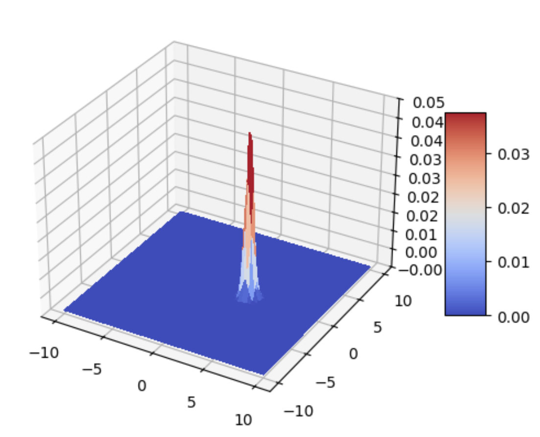
Applying the Schrödinger equation in 2D, we can simulate how a 2D wave function evolves.

However, the calculation for 2D simulation is too complicated for my laptop to run an animation of it. Hence merely an image of the initial state of a 2D wave function is obtained in a relatively low resolution.

1
# Constants
2
x = np.linspace(-10, 10, 100)
3
y = np.linspace(-10, 10, 100)
4
X, Y = np.meshgrid(x, y)

1
class Simulation2D(): # For simplicity, some code's folded up
2
    def __init__(self, phi_0, v):
3
        self.phi = dc(phi_0); self.v = dc(v)
4
        self.dx = x[1] - x[0]; self.dy = y[1] - y[0]
5
        self.lenx = len(phi_0[0]); self.leny = len(phi_0)
6
        self._normalise(); self._hamiltonian()
7

8
    def _normalise(self):
9
        self.phi /= np.linalg.norm(self.phi)
10

11
    def _hamiltonian(self):
12
        """Returns Hamiltonian using finite differences."""
13
        L1 = [[0 for j in range(self.lenx)] for i in range(self.lenx)]
14
        for i in range(self.lenx):
15
            for j in range(self.lenx):
16
                if i == j:
17
                    L1[i][j] = -2
18
                if abs(i-j) == 1:
19
                    L1[i][j] = 1
20

21
        L2 = [[0 for j in range(self.leny)] for i in range(self.leny)]
22
        for i in range(self.leny):
23
            for j in range(self.leny):
24
                if i == j:
25
                    L2[i][j] = -2
26
                if abs(i-j) == 1:
27
                    L2[i][j] = 1
28

29
        # 2D Laplacian using Kronecker products
30
        L1 = np.array(L1) / self.dx ** 2; L2 = np.array(L2) / self.dy ** 2
31
        I_x = sp.sparse.identity(self.lenx); I_y = sp.sparse.identity(self.leny)
32
        L2D = sp.sparse.kron(I_y, L1) + sp.sparse.kron(L2, I_x)
33
        H = (-L2D / 2).toarray()
34
        for i in range(len(self.v)): # Somehow sp.sparse.diags doesn't work qaq
35
            H[i+i*self.lenx] = self.v[i//self.lenx][i%self.lenx]
36

37
        self.H = sp.sparse.csr_matrix(H)
38

39
    def simulate(self, dt = 1e-3):
40
        """Generates wavefunction and time at the next time step."""
41
        U = sp.linalg.expm(-1j * self.H.toarray() * dt)
42
        U[(U.real**2 + U.imag**2) < 1E-10] = 0
43
        phi_flat = self.phi.flatten()
44
        phi_flat = U @ phi_flat
45
        self.phi = phi_flat.reshape((self.lenx, self.leny))
46
        self.phi[self.v > inf-1] = 0
47

48
    def probability(self):
49
        return (self.phi * self.phi.conjugate()).real

1
def gaussian_wavepacket_2D(x0, y0, sigma, p0):
2
    """Gaussian wavepacket at x0 +/- sigma, y0 +/- sigma with average momentum, p0."""
3
    global x, y
4
    return np.exp(1j*p0*x - (((X - x0)**2+(Y - y0)**2)/(2 * sigma**2)))

1
def Free2D():
2
    phi_0 = gaussian_wavepacket_2D(3, 0, 0.5, -1)
3
    V = X*X+Y*Y
4
    o = Simulation2D(phi_0, V)
5
    for i in tqdm.trange(0):
6
        o.simulate(0.5)
7

8
    from matplotlib import cm
9
    from matplotlib.ticker import LinearLocator
10

11
    fig, ax = plt.subplots(subplot_kw={"projection": "3d"})
12

13

14
    # Plot the surface.
15
    surf = ax.plot_surface(X, Y, o.probability(), cmap=cm.coolwarm,
16
                           linewidth=0, antialiased=False)
17

18
    # Customize the z axis.
19
    #ax.set_zlim(-1.01, 1.01)
20
    ax.zaxis.set_major_locator(LinearLocator(10))
21
    # A StrMethodFormatter is used automatically
22
    ax.zaxis.set_major_formatter('{x:.02f}')
23

24
    # Add a color bar which maps values to colors.
25
    fig.colorbar(surf, shrink=0.5, aspect=5)
26

27
    plt.show()
28

29
Free2D()

png

Prospect#

Some improvements could also be made regarding this simulation and animation …

Record physical quantities (momentum, energy, …) during the simulation
Increase the resolution for a higher accuracy
Complete simulations in 2D
…

Thanks for listening ~

Reference#

https://www.astro.utoronto.ca/~mahajan/notebooks/quantum_tunnelling.html

https://docs.manim.community/